2. First steps
2.1. Executing a simulation
2.1.1. With runSofa
💡 To make sure runSofa is able to load a scene described by a python, you can either: * open runSofa without any argument once and then add libSofaPython3 in the plugin manager * or add -l SofaPython3 in this command line.
For more information, please refer to the documentation: Plugin loading.
Once the SofaPython3 plugin is loaded, you can load a simulation from a python script directly in runSofa. Assuming you want to run a script named “example.py”, you can run the following command:
runSofa example.py
Let’s now see how this script example.py should look like.
The first important thing to notice is that to be compatible with SOFA, a python script must define the createScene(root : Sofa.Core.Node) function. This function is the entry point of your simulation and it is automatically called by the runSofa application when a python file is loaded. It is responsible for describing and building the SOFA scene graph.
In the section “Create a new simulation” below, we will detail how to implement this createScene().
2.1.2. With the python3 interpreter
SOFA simulation can also be executed from a python environment (including jupyter notebook).
To do so, the Python environment must be filled in for SOFA python modules.
Located in site-packages/ repositories, the path to these libraries should be added to the PYTHONPATH.
The Installation section details the requirements to execute a simulation withing a python3 interpreter” section details how to configure it.
Once your python environment is properly configured, you will be able to import SOFA python modules (e.g. import Sofa).
By running your simulation from a python interpreter, you will be responsible for:
* creating the root node
* before calling the createScene() function
* and later initializing the graph
Indeed, the python environment does not pre-generate a root node as the runSofa executable is. To be run from a python environment, any python script should therefore look like:
# Required import for SOFA within python
import Sofa


def main():
    # Call the SOFA function to create the root node
    root = Sofa.Core.Node("root")

    # Call the createScene function, as runSofa does
    createScene(root)

    # Once defined, initialization of the scene graph
    Sofa.Simulation.initRoot(root)

    # Run as many simulation steps (here 10 steps are computed)
    for iteration in range(10):
        Sofa.Simulation.animate(root, root.dt.value)
        print("Computing iteration "+str(iteration+1))

    print("Computation is done.")


# Same createScene function as in the previous case
def createScene(rootNode):
    #Doesn't do anything yet
    return rootNode


# Function used only if this script is called from a python environment
if __name__ == '__main__':
    main()
The above script can be run as follows: .. code-block:: shell
python3 example.py
It can be noted that:
* by structuring your scripts this way, you get the advantage to have a script loadable from both runSofa and a python3 interpreter.
* in the above example, the main() function runs 10 time steps without any graphical user interface and the script ends.
Using the SOFA GUI from a python environment
In case you want to manage the simulation from the runSofa GUI, you can call the GUI from the main() function, as follows:
def main():
    # Call the SOFA function to create the root node
    root = Sofa.Core.Node("root")

    # Call the createScene function, as runSofa does
    createScene(root)

    # Once defined, initialization of the scene graph
    Sofa.Simulation.initRoot(root)

    # Import the GUI package
    import SofaImGui
    import Sofa.Gui

    # Launch the GUI (imgui is now by default, to use Qt please refer to the example "basic-useQtGui.py")
    Sofa.Gui.GUIManager.Init("myscene", "imgui")
    Sofa.Gui.GUIManager.createGUI(root, __file__)
    Sofa.Gui.GUIManager.SetDimension(1080, 800)

    # Initialization of the scene will be done here
    Sofa.Gui.GUIManager.MainLoop(root)
    Sofa.Gui.GUIManager.closeGUI()
So far, you can load this python scene, but it doesn’t do much. Let’s enrich this scene!
A scene in SOFA is an ordered tree of nodes representing objects (example of node: hand), with parent/child relationship (example of hand’s child: finger). Each node has one or more components. Every node and component has a name and a few features. The main node at the top of the tree is usually called “rootNode” or “root”. More about how to create a simulation scene can be found in the SOFA online documentation
Using the old Qt GUI
Since SOFA v25.06, SOFA GUI relies on the ImGui library. The previous Qt-based GUI is still available. To use it, make sure to:
add the lib/ repository in the SOFA binaries to your
LD_LIBRARY_PATHadd the lib/python3/site-packages/ repository to your
PYTHONPATHmake sure your SOFA install path does not include any special character
An example using the Qt GUI is available: basic-useQtGUI.py
2.2. Create a new simulation
If a python script is loaded within the runSofa executable, make sure the SofaPython3 plugin is well loaded. When opening the python script, runSofa will search for the createScene(arg0: Sofa.Core.Node) -> Sofa.Core.Node method and it uses it as the entry point of the SOFA simulation, and taking a single parameter: the root Node. Thus define this method:
def createScene(rootNode):
    #Doesn't do anything yet
    return rootNode
2.2.1. Add your first object
We first propose to add a visual grid, in order to see things more clearly. To do that, we simply need to add an object to the rootNode with the right properties :
def createScene(rootNode):
    # Make sure to load all necessary libraries
    import SofaRuntime
    SofaRuntime.importPlugin("Sofa.Component.Visual")

    # Add an object (here of type VisualGrid, with its data "nbSubdiv" and "size")
    rootNode.addObject("VisualGrid", nbSubdiv=10, size=1000)
Now, we create a new child node, in order to add the general configuration of the scene : required plugins (here SofaPython3) and other tools (like a system of axes).
Finally, we add the sphere itself, which consists of two parts : the mechanical representation and the visual representation of the sphere:
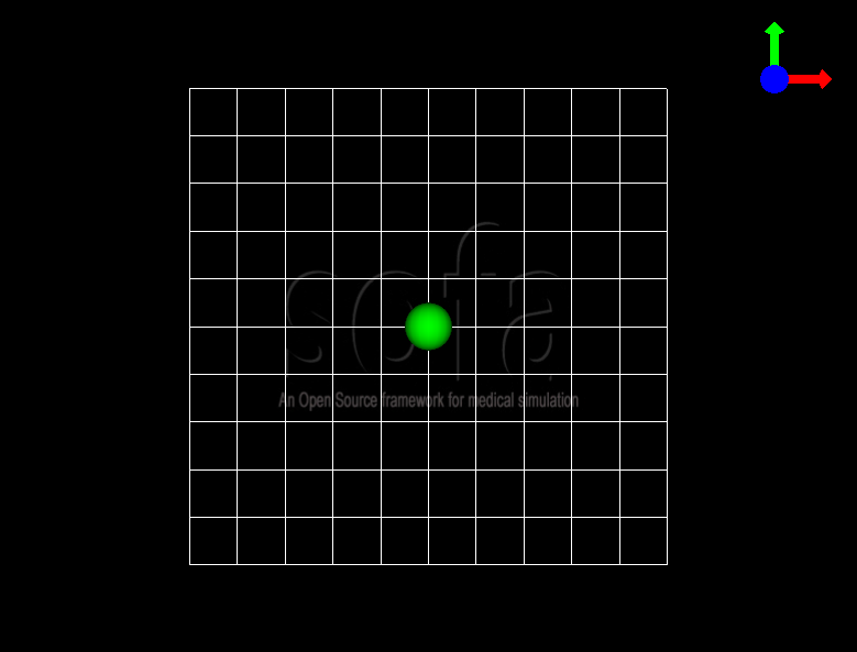
Now, if you execute your scene, you can see a sphere, but it won’t move if you click on the Animate button in SOFA. Let’s change that!
2.2.2. Define physical properties
A default gravity force is implemented on SOFA. Here we reset it, for learning purposes. We also define the time step of the simulation.
rootNode.gravity=[0.0,-9.81,0.0]
rootNode.dt=0.01
We add a mechanical model, so that all our futur elements will have the same total mass, volume and inertia matrix :
totalMass = 1.0
volume = 1.0
inertiaMatrix=[1., 0., 0., 0., 1., 0., 0., 0., 1.]
We add properties to the sphere. First, we add a mass, then an object called ‘UncoupledConstraintCorrection’, in charge of computing the constraint forces of the sphere, then we add two different solvers. One is a time integration scheme that defines the system to be solved at each time step of the simulation (here the implicit Euler Method), the other is a solving method (here the Conjugate Gradient method), that solves the equations governing the model at each time step, and updates the MechanicalObject.
SofaRuntime.importPlugin("Sofa.Component.ODESolver.Backward")
SofaRuntime.importPlugin("Sofa.Component.LinearSolver.Iterative")
SofaRuntime.importPlugin("Sofa.Component.Mass")
SofaRuntime.importPlugin("Sofa.Component.Constraint.Lagrangian.Correction")

# Creating the falling sphere object
sphere = rootNode.addChild("sphere")
sphere.addObject('EulerImplicitSolver', name='odesolver')
sphere.addObject('CGLinearSolver', name='Solver', iterations=25, tolerance=1e-05, threshold=1e-05)
sphere.addObject('MechanicalObject', name="mstate", template="Rigid3", translation2=[0., 0., 0.], rotation2=[0., 0., 0.], showObjectScale=50)
sphere.addObject('UniformMass', name="mass", vertexMass=[totalMass, volume, inertiaMatrix[:]])
sphere.addObject('UncoupledConstraintCorrection')

Now, if you click on the Animate button in SOFA, the sphere will fall.
2.2.3. Add a second object
Let’s add a second element, a floor, to see how they interact :
SofaRuntime.importPlugin("Sofa.Component.Topology.Container.Constant")
SofaRuntime.importPlugin("Sofa.Component.Collision.Geometry")

# Creating the floor object
floor = rootNode.addChild("floor")

floor.addObject('MechanicalObject', name="mstate", template="Rigid3", translation2=[0.0,-300.0,0.0], rotation2=[0., 0., 0.], showObjectScale=5.0)
floor.addObject('UniformMass', name="mass", vertexMass=[totalMass, volume, inertiaMatrix[:]])

#### Collision subnode for the floor
floorCollis = floor.addChild('collision')
floorCollis.addObject('MeshOBJLoader', name="loader", filename="mesh/floor.obj", triangulate="true", scale=5.0)
floorCollis.addObject('MeshTopology', src="@loader")
floorCollis.addObject('MechanicalObject')
floorCollis.addObject('TriangleCollisionModel', moving=False, simulated=False)
floorCollis.addObject('LineCollisionModel', moving=False, simulated=False)
floorCollis.addObject('PointCollisionModel', moving=False, simulated=False)
floorCollis.addObject('RigidMapping')

#### Visualization subnode for the floor
floorVisu = floor.addChild("VisualModel")
floorVisu.loader = floorVisu.addObject('MeshOBJLoader', name="loader", filename="mesh/floor.obj")
floorVisu.addObject('OglModel', name="model", src="@loader", scale3d=[5.0]*3, color=[1., 1., 0.], updateNormals=False)
floorVisu.addObject('RigidMapping')
A floor has now been added to the scene. It is a stationnary object, it won’t move during the simulation. When you click on the Animate button, you can see that the sphere goes through the floor, as if there were nothing there. That is because there is no collision modeling in the scene yet.
2.2.4. Add a collision pipeline
We first add a collision model for the scene in general, that is stating how a contact between the objects is handled: here the objects must not be able to go through one another. Potential collisions are looked for within an alarmDistance radius from the objet. If a collision situation is detected, the collision model computes the behaviour of the objects, which are stopped at a ContactDistance from each other.
# Collision pipeline
rootNode.addObject('CollisionPipeline')
rootNode.addObject('FreeMotionAnimationLoop')
rootNode.addObject('GenericConstraintSolver', tolerance="1e-6", maxIterations="1000")
rootNode.addObject('BruteForceBroadPhase')
rootNode.addObject('BVHNarrowPhase')
rootNode.addObject('RuleBasedContactManager', responseParams="mu="+str(0.0), name='Response', response='FrictionContactConstraint')
rootNode.addObject('LocalMinDistance', alarmDistance=10, contactDistance=5, angleCone=0.01)
We add a new child node to the sphere, that will be in charge of processing the collision.
#### Collision subnode for the sphere
collision = sphere.addChild('collision')
collision.addObject('MeshOBJLoader', name="loader", filename="mesh/ball.obj", triangulate="true", scale=45.0)
collision.addObject('MeshTopology', src="@loader")
collision.addObject('MechanicalObject')
collision.addObject('TriangleCollisionModel')
collision.addObject('LineCollisionModel')
collision.addObject('PointCollisionModel')
collision.addObject('RigidMapping')
We do the same for the floor, but we also specify that the floor is a stationnary object that shouldn’t move.
#### Collision subnode for the floor
floorCollis = floor.addChild('collision')
floorCollis.addObject('MeshOBJLoader', name="loader", filename="mesh/floor.obj", triangulate="true", scale=5.0)
floorCollis.addObject('MeshTopology', src="@loader")
floorCollis.addObject('MechanicalObject')
floorCollis.addObject('TriangleCollisionModel', moving=False, simulated=False)
floorCollis.addObject('LineCollisionModel', moving=False, simulated=False)
floorCollis.addObject('PointCollisionModel', moving=False, simulated=False)
floorCollis.addObject('RigidMapping')
Note that for this step you might have to load the following modules:
SofaRuntime.importPlugin("Sofa.Component.Collision.Detection.Intersection")
SofaRuntime.importPlugin("Sofa.Component.Collision.Detection.Algorithm")
SofaRuntime.importPlugin("Sofa.Component.Collision.Geometry")
SofaRuntime.importPlugin("Sofa.Component.Collision.Response")
SofaRuntime.importPlugin("Sofa.Component.Constraint.Lagrangian.Solver")
SofaRuntime.importPlugin("Sofa.Component.Topology.Container.Constant")
Now, the sphere is stopped by the floor, as it should be. Congratulations! You made your first SOFA scene in Python3!
For more information on how to use the SOFA modules bindings in python, visit this page: Modules
2.2.5. Full scene
Here is the entire code of the scene :
import Sofa
import SofaImGui
import Sofa.Gui


def main():
# Call the SOFA function to create the root node
root = Sofa.Core.Node("root")

# Call the createScene function, as runSofa does
createScene(root)

# Once defined, initialization of the scene graph
Sofa.Simulation.initRoot(root)

# Launch the GUI (imgui is now by default, to use Qt please refer to the example "basic-useQtGui.py")
Sofa.Gui.GUIManager.Init("myscene", "imgui")
Sofa.Gui.GUIManager.createGUI(root, __file__)
Sofa.Gui.GUIManager.SetDimension(1080, 800)

# Initialization of the scene will be done here
Sofa.Gui.GUIManager.MainLoop(root)
Sofa.Gui.GUIManager.closeGUI()


def createScene(rootNode):

    # Define the root node properties
    rootNode.gravity=[0.0,-9.81,0.0]
    rootNode.dt=0.01

    # Loading all required SOFA modules
    confignode = rootNode.addChild("Config")
    confignode.addObject('RequiredPlugin', name="Sofa.Component.AnimationLoop", printLog=False)
    confignode.addObject('RequiredPlugin', name="Sofa.Component.Collision.Detection.Algorithm", printLog=False)
    confignode.addObject('RequiredPlugin', name="Sofa.Component.Collision.Detection.Intersection", printLog=False)
    confignode.addObject('RequiredPlugin', name="Sofa.Component.Collision.Geometry", printLog=False)
    confignode.addObject('RequiredPlugin', name="Sofa.Component.Collision.Response.Contact", printLog=False)
    confignode.addObject('RequiredPlugin', name="Sofa.Component.Constraint.Lagrangian.Correction", printLog=False)
    confignode.addObject('RequiredPlugin', name="Sofa.Component.Constraint.Lagrangian.Solver", printLog=False)
    confignode.addObject('RequiredPlugin', name="Sofa.Component.IO.Mesh", printLog=False)
    confignode.addObject('RequiredPlugin', name="Sofa.Component.LinearSolver.Iterative", printLog=False)
    confignode.addObject('RequiredPlugin', name="Sofa.Component.Mapping.NonLinear", printLog=False)
    confignode.addObject('RequiredPlugin', name="Sofa.Component.Mass", printLog=False)
    confignode.addObject('RequiredPlugin', name="Sofa.Component.ODESolver.Backward", printLog=False)
    confignode.addObject('RequiredPlugin', name="Sofa.Component.StateContainer", printLog=False)
    confignode.addObject('RequiredPlugin', name="Sofa.Component.Topology.Container.Constant", printLog=False)
    confignode.addObject('RequiredPlugin', name="Sofa.Component.Visual", printLog=False)
    confignode.addObject('RequiredPlugin', name="Sofa.GL.Component.Rendering3D", printLog=False)
    confignode.addObject('OglSceneFrame', style="Arrows", alignment="TopRight")
    confignode.addObject("VisualGrid", nbSubdiv=10, size=1000)


    # Collision pipeline
    rootNode.addObject('CollisionPipeline')
    rootNode.addObject('FreeMotionAnimationLoop')
    rootNode.addObject('GenericConstraintSolver', tolerance="1e-6", maxIterations="1000")
    rootNode.addObject('BruteForceBroadPhase')
    rootNode.addObject('BVHNarrowPhase')
    rootNode.addObject('RuleBasedContactManager', responseParams="mu="+str(0.0), name='Response', response='FrictionContactConstraint')
    rootNode.addObject('LocalMinDistance', alarmDistance=10, contactDistance=5, angleCone=0.01)


    totalMass = 1.0
    volume = 1.0
    inertiaMatrix=[1., 0., 0., 0., 1., 0., 0., 0., 1.]


    sphere = rootNode.addChild("sphere")
    sphere.addObject('EulerImplicitSolver', name='odesolver')
    sphere.addObject('CGLinearSolver', name='Solver', iterations=25, tolerance=1e-05, threshold=1e-05)
    sphere.addObject('MechanicalObject', name="mstate", template="Rigid3", translation2=[0., 0., 0.], rotation2=[0., 0., 0.], showObjectScale=50)
    sphere.addObject('UniformMass', name="mass", vertexMass=[totalMass, volume, inertiaMatrix[:]])
    sphere.addObject('UncoupledConstraintCorrection')

    #### Collision subnode for the sphere
    collision = sphere.addChild('collision')
    collision.addObject('MeshOBJLoader', name="loader", filename="mesh/ball.obj", triangulate="true", scale=45.0)
    collision.addObject('MeshTopology', src="@loader")
    collision.addObject('MechanicalObject')
    collision.addObject('TriangleCollisionModel')
    collision.addObject('LineCollisionModel')
    collision.addObject('PointCollisionModel')
    collision.addObject('RigidMapping')

    #### Visualization subnode for the sphere
    sphereVisu = sphere.addChild("VisualModel")
    sphereVisu.loader = sphereVisu.addObject('MeshOBJLoader', name="loader", filename="mesh/ball.obj")
    sphereVisu.addObject('OglModel', name="model", src="@loader", scale3d=[50]*3, color=[0., 1., 0.], updateNormals=False)
    sphereVisu.addObject('RigidMapping')


    # Creating the floor object
    floor = rootNode.addChild("floor")

    floor.addObject('MechanicalObject', name="mstate", template="Rigid3", translation2=[0.0,-300.0,0.0], rotation2=[0., 0., 0.], showObjectScale=5.0)
    floor.addObject('UniformMass', name="mass", vertexMass=[totalMass, volume, inertiaMatrix[:]])

    #### Collision subnode for the floor
    floorCollis = floor.addChild('collision')
    floorCollis.addObject('MeshOBJLoader', name="loader", filename="mesh/floor.obj", triangulate="true", scale=5.0)
    floorCollis.addObject('MeshTopology', src="@loader")
    floorCollis.addObject('MechanicalObject')
    floorCollis.addObject('TriangleCollisionModel', moving=False, simulated=False)
    floorCollis.addObject('LineCollisionModel', moving=False, simulated=False)
    floorCollis.addObject('PointCollisionModel', moving=False, simulated=False)
    floorCollis.addObject('RigidMapping')

    #### Visualization subnode for the floor
    floorVisu = floor.addChild("VisualModel")
    floorVisu.loader = floorVisu.addObject('MeshOBJLoader', name="loader", filename="mesh/floor.obj")
    floorVisu.addObject('OglModel', name="model", src="@loader", scale3d=[5.0]*3, color=[1., 1., 0.], updateNormals=False)
    floorVisu.addObject('RigidMapping')


    return rootNode


# Function used only if this script is called from a python environment
if __name__ == '__main__':
    main()
2.3. Accessing data: read and write
One major advantage of coupling SOFA simulation and python is to access and process data before the simulation starts, while it is running and once the simulation ended. All components in SOFA have so-called data. A data is a public attribute of a Component (C++ class) visible to the user in the SOFA user interface and any data can also be accessed though python.
2.3.1. Read access
Let’s update the Full scene just introduced above in order to access data using the .value acessor once the GUI is closed:
import Sofa
import Sofa.Gui


def main():

...

# Initialization of the scene will be done here
Sofa.Gui.GUIManager.MainLoop(root)
Sofa.Gui.GUIManager.closeGUI()

# Accessing and printing the final time of simulation
# "time" being the name of a Data available in all Nodes
finalTime = root.time.value
print(finalTime)
Note that:
* accessing the Data “time” doing root.time would only return the python pointer and not the value of the Data
* Data which are vectors can be casted as numpy arrays
2.3.2. Write access
In the same way, Data can be modified (write access) using the .value accessor. Here is an example (without GUI) computing 10 time steps, then setting the world gravity to zero and recomputing 10 time steps:
def main():

# Call the SOFA function to create the root node
root = Sofa.Core.Node("root")

# Call the createScene function, as runSofa does
createScene(root)

# Once defined, initialization of the scene graph
Sofa.Simulation.initRoot(root)

# Run the simulation for 10 steps
for iteration in range(10):
        Sofa.Simulation.animate(root, root.dt.value)

# Print the position of the falling sphere
print(root.sphere.mstate.position.value)

# Increase the gravity
root.gravity.value = [0, 0, 0]

# Run the simulation for 10 steps MORE
for iteration in range(10):
        Sofa.Simulation.animate(root, root.dt.value)

# Print the position of the falling sphere
print(root.sphere.mstate.position.value)
The .value accessor works for simple Data structures such as a string, an integer, a floating-point numbers or a vector of these.
For more complex Data such as Data related to the degrees of freedom (e.g. Coord/Deriv, VecCoord/VecDeriv), the .writeableArray() write accessor must be used. Let’s consider a scene graph that would have a ConstantForceField named “CFF” in the sphere node, and that we would like to modify the Data “totalForce” (a Deriv defined in ConstantForceField.h), we should then write something like:
with root.sphere.CFF.totalForce.writeableArray() as wa:
    wa[0] += 0.01 # modify the first entry of the Deriv Data "totalForce"
2.4. More simulation examples
Many additional examples are available within the SofaPython3 plugin in the examples/ folder:
basic.py : basic scene with a rigid particle without a GUI
basic-addGUI.py : same basic scene with a rigid particle with a GUI
emptyController.py : example displaying all possible functions available in python controllers
access_matrix.py : example on how to access the system matrix and vector
access_mass_matrix.py : example on how to access the mass matrix
access_stiffness_matrix.py : example on how to access the stiffness matrix
access_compliance_matrix.py : example on how to access the compliance matrix used in constraint problems
Do not hesitate to take a look and get inspiration!